2 Basic R

The estimated amount of time to complete this chapter is 1-2.5 hours.

In Chapter 1.3 we demonstrated that RStudio can be used as a calculator. The ability to use R as a calculator allows for interactive data analysis. It is important that you learn how to use R for simple calculations before moving on to actual data analysis. This chapter introduces simple calculations in R. In the quiz in Chapter 2.7 you will practice a few calculations.

2.1 R as a calculator

To practice the use of R, run the commands described below while reading the text.

Simple calculations

R can be used as a standard calculator. For example

7 + 11

In the Console Window you will see

> 7 + 11
[1] 18

i.e. a > followed by your command. The result is shown in the line that starts with [1].

NB: If you try copy-paste the line (> 7 + 11) into either the Source or Console window and evaluate the command, you will get an error. This is because the arrow, (>), is not part of the actual code but is a command prompt. Therefore, remember to remove the arrow > at the beginning of the line when copying code from the Console window.

Order of operations

R follows the standard ordering of operations: exponents and roots, then multiplication and divison, then addition and substraction. As usual for calculators, we can use parentheses to change the order. For example, these two lines of code yield different results:

> 10 + 2 * 20
[1] 50
> (10 + 2) * 20
[1] 240

When two operations have the same order, for instance multiplication and divison, R reads the calculation from left to right. We can check this by having R calculate

> 20 / 2 * 5
[1] 50

Here 20 is first divided by 2 and then multiplied by 5 giving the result 50.

Storing values

Values can be stored in variables. Variable names are given by letters or names. Storing is done using an arrow (<-) or simply an equality sign (=). An example of assigning the value of 87 to a variable named age is:

age <- 87

or

age = 87

To see the content of the age variable simply type

> age
[1] 87

The stored values can be used for calculation:

> age + 2
[1] 89

When assigning values to variables, the variables will appear in the Environment window along with their value. Variables can only be named using numbers, letters from A to Z, period “.”, and underscore “_" and may not start with a number. Space is not allowed in the name and each name is case-sensitive, such that Age and age are two different variable names.

Storing values can be really handy when you need to do further calculations on a value.

Now watch the video (3 min) below illustrating some of the topics covered so far (click the HD-button at the lower right corner of the video to view in highest possible solution):

Click here to find the code produced in the video

# R as calculater
1+5
3*(1+5)/(4+2^2) 
3*1+5/4+2^2 # order of operations

# some more
log(5)
exp(5)
sqrt(5)

# store simple values 
y <- sqrt(5)
y
5/y
y*2
Y # case sensitivity

---

Contents of the video:

R can be used as a calculator and it uses the same signs as other calculators: + (addition), - (subtraction), * (multiplication), / (division) and ^ (raise to power).

2.1.1 Activity

Activity 1

Determine the value of \(\frac{1.27^2+2.04^2}{2}\).

Test your result here

The result is 2.8875, (1.27^2 + 2.04^2) / 2. Be careful with the parentheses, otherwise your result will be wrong!

---

Activity 2

To divide the number 1 with 4, which syntax do you need?

1/4 or 1:4?

Test your result here

The correct answer is: 1/4

The sign / is used for division in R. The : sign in this context will result in a sequence of numbers with values from 1 to 4. Such a sequence is also termed a vector (vectors are described in more detail in Chapter 3.2). Another example is e.g. 3:10 which results in the sequence 3, 4, 5, 6, 7, 8, 9, 10. Hence it is a sequence from 3 to 10 by steps of size 1. Sequences are very useful in R as will be be demonstrated in the following chapters.

---

Activity 3

What will be the output of the following code?

a <- 9
b <- 3
A/b

Test your answer here

The answer is: Error: object ‘A’ not found.
If you have set the language to Danish the answer is: Fejl: objekt ‘A’ blev ikke fundet.

R is case sensitive. This means that if you have defined a, it will not be able to find A. As you have not defined A, R is not able to find it and gives you the error message in the console: Error: object ‘A’ not found.

Instead use a/b.

---

2.2 Mathematical functions

In addition to the basic arithmetic operations, R has built-in standard mathematical functions. The following list includes the most commonly used mathematical functions:

Function	Explanation	Example
abs(x)	Absolute value	abs(-3)=3
sqrt(x)	Square root	sqrt(9)=3
a^x	Power function, a raised to power x	2^3=8
exp(x)	Exponential function	exp(1)=2.718
log(x)	Natural logarithm (base e=2.718)	log(10)=2.303
log10(x)	Logarithm base 10	log10(10)=1
log(x, base=b)	Logarithm base b	log(8,base=2)=3

For example, to determine the square root of 2 we use:

> sqrt( 2 )
[1] 1.414214

2.2.1 Activity

Determine the value of log(1).

Test your result here

The logarithm of 1 is 0, no matter the base (log(1)=0=log10(1)=log(1,base=2).

---

2.3 Functions

In the previous two chapters, 2.1 and 2.2, we introduced some of the mathematical functions in R. When working with R we use functions whenever we want R to do something (calculations, loading data, plotting, …). We will also refer to these functions as commands and use the words functions and commands interchangably.

Any function in R is used by writing the name of the function and parsing it the necessary arguments. The function will then return a result based on the arguments. The structure is:

functionName(argument1, argument2, ...)

The number of arguments needed, their order in the list of arguments and the class/type of the arguments depend on the specific function. For example the syntax of the log() function is:

log( x, base )

meaning that the log-function accepts up to two arguments, x the value we want to determine the logarithm to and base specifying the base with respect to which the logarithm is computed.

A lot of commands need only the first argument, here for example

> log( 5 )
[1] 1.609438

or equivalently

> log( x=5 )
[1] 1.609438

Suppose we want to determine the logarithm to 5 with base 2. We may use:

> log( 5, 2 )
[1] 2.321928
> log( x=5, base=2 )
[1] 2.321928

When omitting the name of the arguments (here x and base) we have to be very careful with the order in which they appear (log(5,2) is not the same as log(2,5)). However if we specify the names of the arguments, log( x=5, base=2 ) and log( base=2, x=5), the order is irrelevant.

All R commands need the first argument and we therefore often supress the name of the first argument but as some R commands have many extra arguments, we typically specify the names of these to avoid remembering the order (and yes, you will learn the names of some of the most common arguments by heart). For the logarithmic function we would therefore specify the command as:

log( 5, base=2 )

2.4 Combination of functions

It is possible to combine functions, namely to use the output of one function as the input to another. To determine the value of \[ \exp( \, \sqrt{ 1+ 0.7\times\log_2(5)^3} \, ) \]

we may simply write

> exp( sqrt( 1 + 0.7*log(5, base=2)^3 ) )
[1] 22.74971

Another way around would be to successively store values:

> v1 <- log(5, base=2)
> v2 <- v1^3
> v3 <- 1+0.7*v2
> v4 <- sqrt( v3 )
> v5 <- exp( v4 )
> v5
[1] 22.74971

Due to rounding error we will avoid doing calculations stepwise as:

> log(5, base=2)
[1] 2.321928
> 2.32^3
[1] 12.48717
> 1+0.7*12.487
[1] 9.7409
> sqrt( 9.74 )
[1] 3.120897
> exp( 3.12 )
[1] 22.64638

2.5 Autocorrect and code autocompletion

R has no autocorrect

If you make a typo while using R, the program will not try to “guess” which command you were trying to write. If we instead of log(5) wrote e.g.

> Log(5)
Error in Log(5): could not find function "Log"

we get an error message. Always pay attention to the error message as often (not always!), the error message can help us correct the error. Here R tells us that it cannot find a function named Log because there is no log-function with a capital L.

We (generally) do not have to worry about spacing when working with R. Thus the following two lines of code will yield the same result

> 1+10
[1] 11
>     1    +   10
[1] 11

There are, however, exceptions. For example, spaces in function names does not work:

> lo g(5)
Error: unexpected symbol in "lo g"

Note that R tells that there is an unexpected symbol, namely a space, in the function name.

Similarly we (generally) do not have to worry about line breaks as the code below is evaluated correctly :

1 + 

  10

[1] 11

However, we have to be a bit careful as it not the same as

1 

  + 10

that evaluates to

[1] 1
[1] 10

The difference is that in the first of the two calculations of 1+10 above, the + following the 1 indicates that the calculation is not finished yet. R therefore waits for further numbers to be added. In the second calculation R evaluates the number 1 to 1 and has no chance of figuring out that more lines will appear later on. Secondly ‘nothing’ +10 is evaluated as 10.

Similarly we may add line breaks or spaces when applying functions, e.g. calculating log(5,base=2) as

log( 5     ,
     base=2
     )

[1] 2.321928

Sometimes we unintendedly submit code that is not complete. Suppose we wanted to calculate 2 * 20 / 5 but pressed Ctrl+Enter after writing only

2 * 20 /

This would yield the following output in the Console

> 2 * 20 /
+ 

Here + indicates that R needs further information to complete the calculation (here the number 5). If we now write 5 and press Enter in the Console we get the correct result. This issue of not having completed the calculation often occurs when working with quotation marks or parentheses, e.g. when not having the same number of left and right parantheses (unbalanced parentheses). In these cases it can be difficult to pinpoint exactly what is missing, and it is often useful to cancel the calculation and spend some time looking at the code and adding the missing parts. To cancel an unfinished calculation, simply press Esc in the Console window.

2.5.1 Activity

Copy the code below to your Script, press Ctrl+Enter to submit the command. Note the + that appears in the last line of the Console, indicating that R waits for more input. Now cancel the calculation by moving the cursor to the Console window and pressing Esc.

((2 + 1) / ((2 - 5) + 1) * (5 + 3)

What is wrong with the above code?

Solution

There is an unbalanced paranthesis, namely 5 left parantheses and only 4 right parantheses. A way to finish the calculation is therefore to add an extra right paranthesis: Again evaluate the above line and when the expression

> ((2 + 1) / ((2 - 5) + 1) * (5 + 3)
+ 

occurs in the Console window, type a ) followed by Enter in the Console window. If you copied the command to your script, don’t forget to correct the code in the Script window such that it can be evaluated without errors next time you open your script. You can correct the code by adding a ) at the end of the expression or by deleting the redundant ( at the beginning of the expression, i.e.

((2 + 1) / ((2 - 5) + 1) * (5 + 3))

or

(2 + 1) / ((2 - 5) + 1) * (5 + 3)

---

Autocompletion

RStudio supports automatic completion of code using the ‘Tab’ key. For example, if you want to calculate the square root of a number (which is done using the command sqrt()) you can start by typing e.g. sq, pressing ‘Tab’ and RStudio will provide a list of matching suggestions. You can use arrow up / down to browse between the suggestions and you select the suggestion highlighted in blue by pressing ‘Enter’:

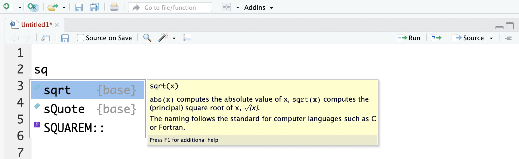
Figure 2.1: Autocomplete searching for square root function using the ‘Tab’ key.

Note that RStudio also gives a short description of the function in the yellow box to the right of the suggestion.

You may also use autocomplete to help with the names of the arguments. If you, inside the parentheses of a function press the ‘Tab’ key, RStudio will provide a list of the possible argument names - along with a description of the argument (yellow box):

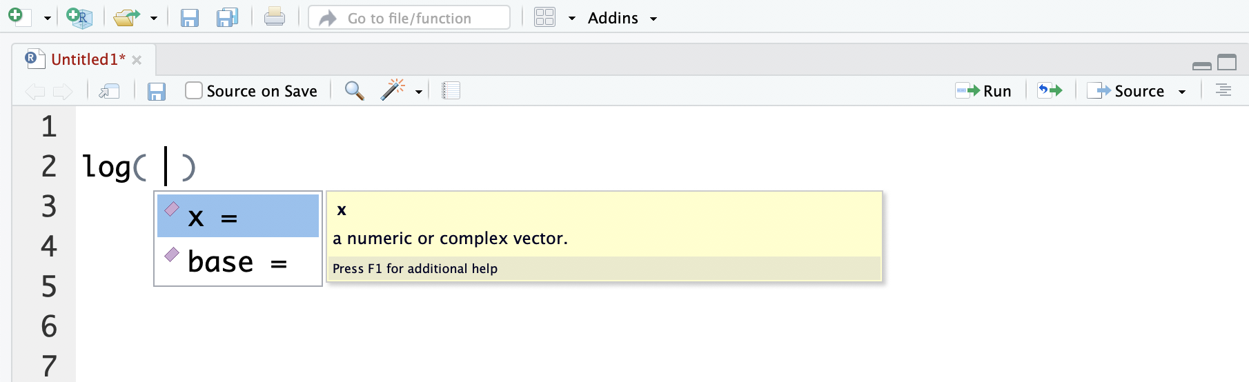
Figure 2.2: Autocomplete searching for the names of arguments to the log function using the ‘Tab’ key.

2.6 Help

When using functions in R, we might need help to find out which arguments to use. Here we may use the help function (help()). To find out which arguments to use in the log() function we specify:

help( log )

Running this command results in the help page for Logarithms and Exponentials appearing in the Files/Plots/Packages/Help/Viewer window.

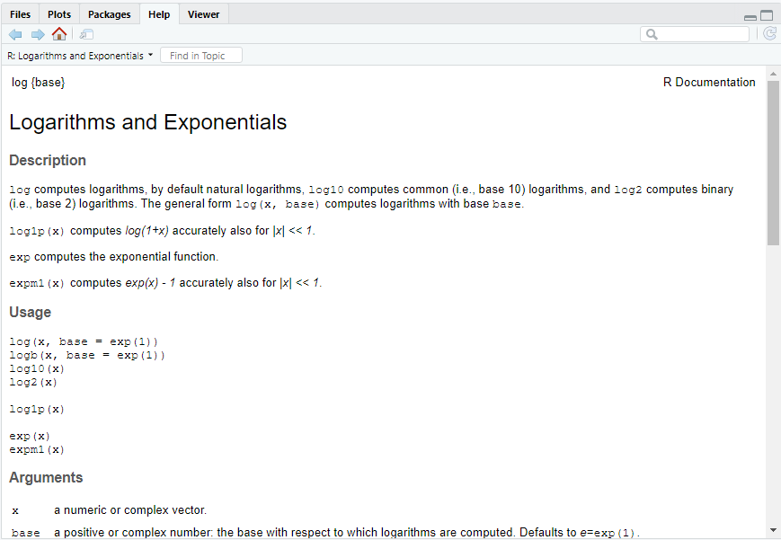
Figure 2.3: The help page for Logarithms and Exponentials.

This help page is general for all logarithms and exponentials. It begins by describing the different functions (Description), then gives examples of how to use the functions (Usage), and then lists the names of the arguments along with a description of their types (Arguments). We find that the arguments, x and base, not surprisingly, should be numbers (numeric or complex) and that the base has to be positive. A Details section given further down (not included in the Figure) gives a general and often technical description of the function and how it operates. A Value section gives a description of what the function returns. At the bottom of the help page you always find Examples demonstrating how to use the functions. You can try evaluate the code given to explore how to use the functions.

You may of course also google to find help on the use of R functions. Simply goggle “R log” or “R logarithm”. As a new R user, however, it can be difficult to find the information on the web - and you probably also find the built-in help pages (help()) difficult to read. Instead you can use the Appendix B which contains a list of some of the most commonly used functions including a short description of their use. As you obtain experience using R you will find it easier to google or to use the help pages.

2.7 Additional activities

Here you find 4 activities to further explore the use of R as a calculator.

Activity 1

Is the result of 0.5/2 identical to the result of .5/2?

Test your result here

True. We may omit the zero before the decimal point.

---

Activity 2

Use the == operator to check if 0.5/2 is equal to .5/2:

0.5/2 == .5/2

What is the output created by R?

Test your result here

The answer is TRUE. Had the expressions not been equal the output would have been FALSE. R operates with TRUE and FALSE values. Note that a single equality cannot be used to test whether two numbers are equal, 0.5/2 = .5/2 will not work (try and you will get a strange error message). In general, single equality is used to specify values for function arguments or it may be used instead of the assignment operator (<-). I.e. these two expression both assigns the value 17 to an object named x:

x <- 17
x = 17

---

Activity 3

Use the round() function to round off \(\pi\) (3.142) to the nearest integer value. Next use the help pages (help(round)) to find out how to round \(\pi\) to two decimals.

Test your result here

The nearest integer value is 3 which may be found using the command round(3.142).
The help-page contains information on several functions to be used for rounding of numbers. We focus on the round() function and find in the Usage section that round() takes an additional argument digits that, according to the Arguments section, is an integer (a whole number) indicating the number of decimal places. I.e. to round to two decimals, we may use round( 3.142, digits=2) (or simply round( 3.142, 2) since digits is the second (and last) argument).
Note that instead of entering the number 3.142 we may use that the number \(\pi\) is defined in R and use:

> pi
[1] 3.141593
> round(pi)
[1] 3
> round(pi,2)
[1] 3.14

---

Activity 4

Having completed Activity 3 you might have noted that several other rounding functions are available. By applying the functions ceiling(), floor() and trunc() to \(\pi\) and -\(\pi\) and / or reading the help-page - what do these functions do?

Test your result here

The ceiling() function rounds to the upper nearest integer value (i.e. results are 4 and -3 for ceiling(pi) and ceiling(-pi), respectively).
The floor() function rounds to the lower nearest integer value (i.e. results are 3 and -4).
The trunc() function rounds to integer values towards 0 (i.e. results are 3 and -3).

---