1 R and RStudio
The estimated amount of time to complete this chapter is 45-60 minutes.
R is a free open source software program for statistical analysis. R is command based, meaning that the user types a command (also denoted code) and R will compute and display the results. RStudio is a user interface to R and we will be working with R from RStudio only. In this chapter we first describe how to install the two programs. Next we give guidelines on how to organize and name the files on your computer. Finally we demonstrate how to interact with RStudio by showing a few simple calculations. At the end of Chapters 1.2-1.4 you find small activities to explore the RStudio interface a bit further than described in text and videos.
1.1 Installation of R and RStudio
Install R:
- Visit R’s webiste and click on CRAN under Download located in the left pane
- Choose a location near you (Denmark) in the appearing scroll-down menu.
- Click on one of the links: Download R for MacOS, Download R for Windows or Download R for Linux, depending on your operation system.
The following steps are for Windows users:
- Click on install R for the first time placed in the text related to base.
- Click on Download R x.x.x for Windows (x.x.x indicates the version of R)
- Follow the installation Wizard
The following steps are for Mac users:
- Click on R-x.x.x.pkg - choose the link with the highest version number that supports the version of your operation system. The version supports are mentioned under the “Latest Release” pane.
The following steps are for Linux users:
- Click on the link corresponding to your distribution of Linux.
- Follow the instructions in README.
Install RStudio:
- Visit RStudio’s Download page and click the appropriate link under Installers that correspond to your operation system and version.
You may now open RStudio. How to interact with RStudio is explained in Chapter 1.3 below. Before you start working with RStudio we recommend that you set up a folder (in Danish: mappe) with subfolders for storage of files on your computer:
1.2 Folder structure
During your statistics course and when working on your own data, you will be working with many different files: data files, files containing R code, reports and files containing background material. To avoid having a mess of files on your computer you should save the files used during the course in one folder. To further structure the contents of the folder, we recommend that you define four subfolders named data, code, report and material for storage of:
| Folder name | Content | File type |
| data | Data files | .csv, .csv2, .txt, .xlsx etc. |
| code | R code files | .R |
| report | Reports | .docx, .pdf, .Rmd etc. |
| material | Background material, lecture notes, explanatory solutions etc. | .docx, .pdf, .pptx, |
For this online introduction, you may define a folder named e.g. Rintrocourse in your Documents folder (NB: don’t use spaces in folder names, more details below). Having defined the four subfolders in the Rintrocourse folder, using Finder (Mac) (or Explorer on Windows) the folders are shown as:
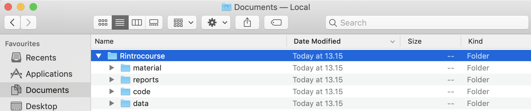
Figure 1.1: The folder structure shown on a Mac.
If you need help on how to define the folders on your computer, click here
Mac users: Open Finder (click the Finder icon in the Dock).
Windows users: Open Explorer (Stifinder).Click on your Documents folder (probably shown under in the sidebar to the left).
In the Documents folder, press Command-Shift-n (Mac) / Ctrl-Shift-n (Windows). A new folder appears with suggested name ‘Untitled folder’ (‘Ny mappe’). Enter another name for the folder, e.g. Rintrocourse.
Enter the new folder (click on the folder).
Add a new folder (Command-Shift-n / Ctrl-Shift-n) and name the folder data. Similarly define the other three folders in the Rintrocourse folder.
When you start working with another course or your own data, you should define a similar folder with subfolders for storage of your files.
Naming files and directories
Two keys to good naming are consistency and descriptiveness. The names need not necessarily be long to fulfill the two characteristics. Often the task of naming is easier when files are already stored in a directory structure like the one presented above as the files are already associated with the name of the folder.
Concatenating names
When you name a folder or a file the name may consist of separate words. E.g. for a data set concerning tumors in mice the words mice and tumor may be good descriptive words for the data set. Ways of concatenating the names are then:
- Underscores or dashes: mice_tumor.xxx or mice-tumor.xxx
- No seperation: micetumor.xxx
- CamelCase or pascalCase: MiceTumor.xxx, miceTumor.xxx
Please notice that ‘mice tumor.xxx’ is not listed as a good way of naming a file containing multiple words. We recommend to never ever use space in file or folder names as this may create technical challenges in some settings.
Special Characters
Special characters such as: ~ ! @ # $ % ^ & * ( ) ` ; < > ? , [ ] { } ’ " and | must be avoided in naming. Special language characters should also be avoided (e.g. æ, ø, å). If it is most meaningful to name in ones own language, substitute the special language characters to the English letters (e.g. å to aa, æ to ae etc.)1.2.1 Activity
Before you move on to the next chapter: Define a new folder on your computer containing the four subfolders.
1.3 The RStudio interface
RStudio is a user interface to R consisting of four windows. In the video below the two most important windows, the Source and the Console window, are explained (3:30 min):
To watch the video in highest possible resolution, use the gear icon at the bottom of the video. The quality of the videos should be fine and if you experience bad resolution of the videos and cannot change the resolution, you might need to update your browser or try using another browser (e.g. Chrome). You can also increase the playback speed using the gear icon.
Contents of the video
The first time you open RStudio, three windows will be presented. A fourth window, the Source window, is opened by pressing the File drop-down menu -> New File -> R Script.
Window 1: Source
The Source window contains R code. A line of code in the Source window can be passed to the Console window by placing the cursor at an arbitrary location in the line and pressing Ctrl-Enter or Ctrl-r (on Mac Command-Enter).
Lines with comments start with a hashtag (#).
Lines of code you want to save should be written in the Source window and saved as an R file (also denoted an R script, see how in activity below).
Window 2: Console
In the Console window, code is compiled and the results are printed. The code can be directly entered in the Console by typing the code and pressing Enter. Alternatively it may be submitted from the Source window as described above.
In the video below, the remaining two windows are explained (2:30 min). First, however, we show how to save values in variables:
Contents of the video
How to define variables (also termed objects) containing values is described en more detail in Chapter 2.1.
Window 3: Environment/History/Connections
The most important tab in this window is the Environment tab. The Environment is an interactive list of R objects (values, vectors, data frames etc.). All the objects you define during your session will appear in the list. The History tab contains all commands executed during a session.
Window 4: Files/Plots/Packages/Help/Viewer
In the Files tab you can browse through your files and you may open your R script files from here (you may also do that using the drop-down menu File -> Open File). The Plots tab will show the plots you produce, Packages will contain a list of the packages you have installed (more on packages later), Help contains help pages and Viewer can be used to view local web content. Typically we only use the Plots and Help tabs.
1.3.1 Activity
Before you move on to the next chapter: Save the commands showed in the video in an R script:
Open a new R script using the menu File -> New File -> R Script.
Either type in the commands used in the two videos above or copy the lines to your Source window:
# Adding numbers
4+5
2+3

age <- 87
oldage <- age + 2
sumage <- age + oldage

gender <- "male"
Evaluate the code line-by-line by first placing the cursor at an arbitrary position in comment line and pressing Ctrl-Enter (Command-Enter on Mac). As the cursor moves to the next line, you can run the program line-by-line by pressing Ctrl-Enter until you reach the last line. Continue with the remaining lines of code. Note that the four variables appear in your Environment window.
You should save the commands in the Source window in an R-file (also denoted an R-script), namely a file with suffix .R in the file name: Use the menu ‘File’ -> ‘Save As’ and browse to your subfolder named code and name the file e.g.
Chapter1_RStudio_Windows.R. A pop-up box asking you to choose the encoding might appear in which case you simply choose the first option (UTF-8). Note that the file name now appears in the tab in top left of your script window. The contents of an R-script is also referred to as a program.At the bottom of the file, enter a new line, e.g.
meanage <- sumage / 2. Note that, while changing the file, the colour of the file name in the top left change from black to red and an asterix (*) is placed to the right. Now save the file by pressing Ctrl-s (Command-s on Mac) or use the menu File -> Save. The file name colour changes to black and the asterix disappears. It is a good habit to constantly save your script as your changes may be lost if R crashes.
1.4 Quitting RStudio
Your R workspace includes all the objects you have defined while working in R. These are listed in your Environment tab and typically you will generate a lot of objects (like the values colour and y defined above). Usually we are not interested in saving all these objects as the objects easily can be generated again by running the commands in your R script.
Like most other programs, RStudio can be quit by pressing the X in the top right corner of the window (top left on Mac). When quitting R, you will be asked whether you want to “Save workspace image” which you generally don’t want to. To permanently tell RStudio not to ask whether to “Save workspace image” you may change your preferences using the menu Tools -> Global Options and set “Save workspace to .Rdata on exit” to “Never” as illustrated in Figure 1.2:
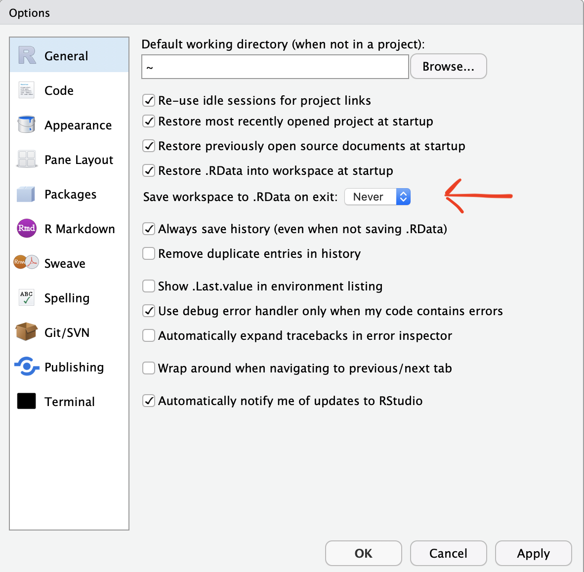
Figure 1.2: The window used to change preferences, here specifying that R should never promt whether to save the workspace on exit.
1.4.1 Activity
Before you move on to the next chapter: Study the objects in the Environment tab, learn shortcut keys and try quit RStudio:
In the Environment tab - what happens when you press the small brush (below ‘Connections’)? Choose ‘Yes’ in the pop up box.
Redefine the five variables
age,oldage,sumage,genderandmeanagein the Environment by running your R script again.- Suppose we made an error and
genderwas supposed to be set to"female". Add an extra line to the bottom of your program specifyinggender <- 'female'(note you may use single or double quotes). Now again run your program line-by-line - meanwhile pay attention to the Environment window. What happens to the value ofgenderwhen you run the last line?
Did you note that the value of-
Test your answer here
gendershown in the Environment tab changed from'male'to'female'when running the last line? This means that the value ofgenderis overwritten. Instead of having two separate lines defininggenderwe will only keep the line we need (gender <- 'female') in our program. Therefore, delete the line containinggender <- 'male'from your script. Place the cursor at an arbitrary position in the Script window. Press Ctrl-2 - what happens to the cursor? Now type
2+3in the Console window followed by Enter. Press upwards arrow - what happens? Modify the calculation to2+7(use the backspace key) and press Enter. Press upwards arrow twice - which command appears?
Press Ctrl-1 to have the cursor placed in the Script window again.Save your program (Ctrl-s) and quit RStudio (without saving the ‘workspace image’). Open RStudio again and run the complete program. What do you find in your Environment?
In this activity you were introduced to some of the shortcuts in RStudio. Many more are available: Type Alt + Shift + k (Option + Shift + k on Mac) for a complete list.