4 Data import and export
The estimated amount of time to complete this chapter is 1-2 hours.
This chapter is important! We are working with several data files in our courses in biostatistics. If you cannot load data into R, you will not be able to perform any analyses. Loading data is a bit technical and we therefore recommend that you study this chapter carefully and spend some time playing around with the different data files to be sure that you will be able to load data when your course starts.
There are various different formats for storage of data and depending on the format, the data has to be loaded into R in different ways. In this chapter you will be introduced to CSV and text files which are common formats for storing of data files in our courses.
The steps involved when loading data into R are
- Download the data file to your data folder (Section 4.1).
- Tell R in which folder you saved the data (Section 4.2).
- Load the data into R (Sections 4.3 and 4.5).
- Examine whether the data were loaded correctly (Section 4.4).
4.1 Data file formats and download
To avoid problems when loading the data into R it is important to be aware of the format of the data file and where it is located on your computer. In this chapter we explain the difference between some typical data files and how to download them to your folder.
We will be working on a sub sample of data from a large study of health in Copenhagen. The study is named SundBy (Sund=Healthy, By=City) and contains an id number (id), gender (gender, code 1 for males), height (ht, in cm) and weight (wgt, in kilos) for 200 individuals. The data thus contains 200 rows and 5 columns of which the first 6 rows are shown in the table below:
| id | gender | age | wgt | ht |
|---|---|---|---|---|
| 1434 | 2 | 31 | 70.0 | 172 |
| 978 | 1 | 28 | 68.0 | 170 |
| 701 | 2 | 55 | NA | 165 |
| 134 | 1 | 26 | 76.0 | 180 |
| 292 | 2 | 21 | 60.0 | 175 |
| 1481 | 2 | 27 | 61.5 | 178 |
Note that the third individual, a female with id number 701, has no registration of weight. The code for missing value is NA (Not Available) in R. Further note that the weight variable (wgt) has decimal values as person with id 1481 is registered with a weight of 61.5 kilos.
Text data files
The data files we provide in our statistics courses are often text data files. These are stored as CSV or text files (file name extensions .csv resp. .txt). The filename extension tells you which format the data is stored in.
-
CSV is short for Comma Separated Values. Excel reads CSV-files and you may also export CSV-files from Excel. Data is stored in plain text. If the CSV file is exported from an English version of Excel, the values in each line will be separated by commas (,). If the CSV-file is generated using a Danish version of Excel, comma is used for decimal places and the values are separated by semicolons (;). More details on English / Danish CSV files are given in Chapter 4.3 below.
- Text files are similar to CSV files, the difference being that values are separated by spaces or tabs. More details on text files are given in Chapter 4.5.
Download
You find three versions of the SundBy data set here, namely two CSV-files (sundby0_English.csv, sundby0_Danish.csv) and a text-file (sundby0.txt).
First you need to download the files to your computer: Define a folder on your computer with the files you are using for this introduction. Name it e.g. Rintrocourse. In this folder, define a folder named data (as suggested in Chapter 1.2). Download all three SundBy files to the data folder. Open the folder (using Explorer (Stifinder) on Windows, Finder on Mac) in list view to see that the files were downloaded correctly:
On a Windows computer the contents of the folder should look like this:
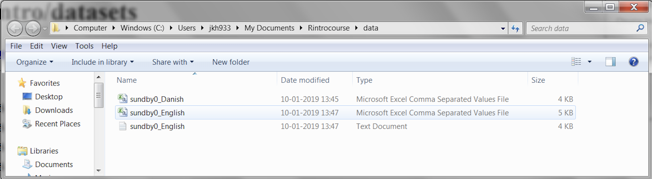
Figure 4.1: The folder contents shown on a Windows computer with correctly downloaded SundBy data files.
On a Mac the contents of the folder should look like this:
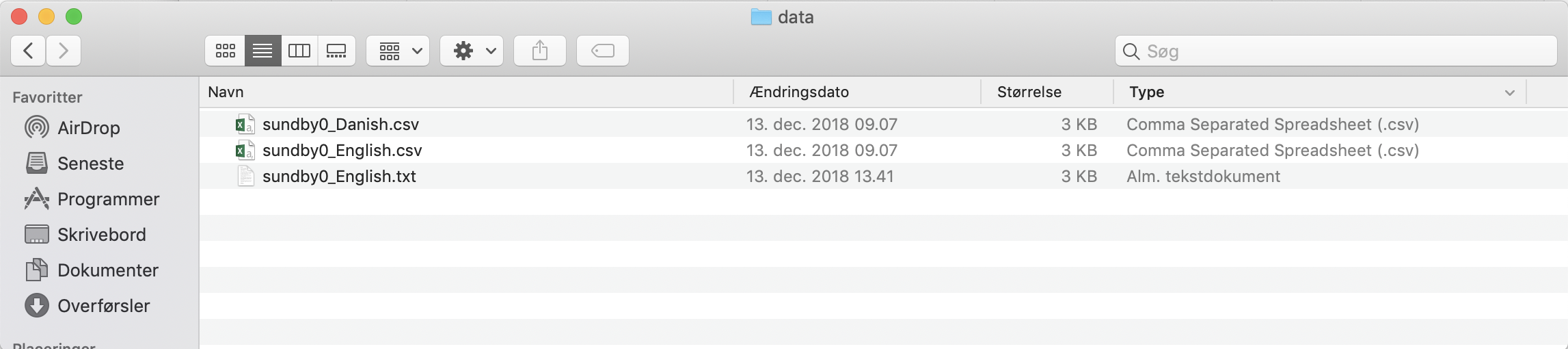
Figure 4.2: The folder contents shown on a Mac with correctly downloaded SundBy data files.
The type of the files is listed in the column named “Type” as the content of the folder is shown in list view. The file types are shown as “Comma Separated Values / Spreadsheet” respectively “Text Document” indicating that the files were correctly downloaded. Also note that the files have different icons to the left of the file names.
Before you move on to the next chapter: Download the three data files to your data folder. Make sure that you have got the file types correct - if so, you may skip the rest of this chapter and go straight to Chapter 4.2.
If the content of your folder looks different with respect to the type of the files, the files were not downloaded correctly. You will therefore have to download the data files in another way:
How to download data files
If you use Explorer as your browser you may experience that all files appear to be html files. That will not work! Instead you will have to download the files in a different way:
Use Chrome as your browser. You can download Chrome from here. There are two different ways to save the files on your computer from Chrome:
- Right click on each of the files and choose ‘Save link as’. Browse to your folder and click save.
-
Left click on the file. Chrome will either:
- Start downloading the file and when the download has finished, it will appear in the download bar at the bottom of the page. Click on the small arrow next to the file tile and select ‘Show in folder’. The file is showed in your Downloads folder and from here you can move it to your data folder.
- If the file is a text file, Chrome might choose to show you the file / open the file in the browser. In this case, go back to the page with the list of the files (using the arrow to the left at the top of the page next to the URL). Follow the steps described in A. using right click.
4.2 The working directory
Having downloaded the data files you need to tell R in which folder to find the data. This folder is termed the working directory. How to define the working directory is shown in this video (3:11 min):
Contents of the video:
The working directory is set using the menu Session -> Set Working Directory -> Choose Directory. Browse to the folder with the data files. This will cause R to generate a command setwd() (set working directory) specifying the path to the folder:
# NB: Your path will be different than mine, depending on the names of your folders
setwd( '~/Documents/Rintrocourse/data/' )
Instead of using the menu, you may use the setwd() command to set the working directory. To see the contents of the folder you may use the command dir() (directory). Having downloaded the three SundBy data files to the folder, the contents will be:
> dir()
[1] "sundby0_Danish.csv"  "sundby0_English.csv" "sundby0_English.txt"
Rstudio now knows where to locate your data files as well as the names on the files.
Tip: Copy the setwd() command with the path to your folder from the console window to your script. Next time you open the script you can define the working directory by evaluating this command instead of using the menu.
If you are in doubt about which folder R considers as your working directory you can use the command getwd() (takes no arguments).
Before you move on to the next chapter: Set your working directory to the folder containing your data files. Next use the dir() command to see that the three data files are located in your working directory.
4.3 Loading CSV files
Prior to importing a data file of .csv/.txt format it is useful to know:
- How are the values separated: semicolon (;), comma (,), tab (), or perhaps blank (‘’)?
- Does the first row contain variable names (a so-called header)?
- Are missing values listed with a word, number or special characters?
- Are decimals numbers listed using periods (.) or commas (,) corresponding to the English or Danish symbol for the decimal separator?
A way to find out is simply by opening and studying the file in Notepad on Windows / TextEdit on Mac.
Loading English CSV files
In the file named sundby0_English.csv data are stored in English format, i.e. with English decimal number (period) and values separated by commas. A snapshot of the file (using Notepad on Windows / TextEdit on Mac):
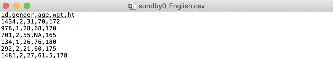
Figure 4.3: A snapshot of the SundBy CSV file saved in English format.
We note that the first line is a header, namely a row containing variable names, and that the missing value code is NA. Also note from the 6th data line (id 1481) that the decimal point is a period.
CSV files in English format are loaded in to R using the command read.csv(). This command takes as input the name of the datafile (surrounded by quotes). To save the data in a data frame named d we specify
d <- read.csv("sundby0_English.csv")In your Environment tab you should now find an object named d with 200 observations of 5 variables.
How to load the data and a few more explanations is given in the video below (4:00 min):
If you get an error message Error in file(file, “rt”) : cannot open the connection you either misspelled the file name or the file is not located in the working directory. Check your spelling and the contents of your working directory (using dir()) and run the command again after you have changed the spelling / changed the working directory / saved sundby0_English.csv in the folder. The video below gives some more details on how to find out what is wrong (4:20 min):
Loading Danish CSV files
In the file named sundby0_Danish.csv the data are stored with Danish decimal number, i.e. a comma is used as the decimal point and the values are separated by semicolons. A snapshot of the file (using Notepad on Windows / TextEdit on Mac):
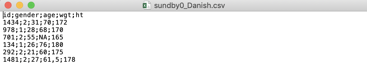
Figure 4.4: A snapshot of the SundBy CSV file saved in Danish format.
CSV files in Danish format are loaded in to R using the command read.csv2() (make sure the working directory is set before evaluating the command):
d <- read.csv2("sundby0_Danish.csv") Before you move on to the next chapter: Load the SundBy data into a data set named d (using either the English og Danish version).
4.4 Exploring the data
When data have been loaded it is important to examine whether the data were properly loaded and to explore features of the data. R provides several commands that allows us to examine the data, the table below giving some of them:
dim()
|
The dimension of the data frame (number of rows and columns) |
names()
|
The names of the variables in the data frame |
head()
|
Print the first 6 lines of data |
tail()
|
Print the last 6 lines of data |
View()
|
View the data in spreadsheet style in new tab in the script window. You may also double click on the data object in the environment window |
str()
|
A compact overview of the data including the types of the variables and the values of the first 10 rows in the data set. |
summary( d )
|
A summary of all variables in the data set. Descriptive statistics such as mean and median are given for all numeric variables whereas categorical values are tabulated (first 5 categories only). |
The video below illustrates how to use some of these command to explore the SundBy data set (4:41 min):
Click here to find the code used in the video.
# see Chapter 4.1-4.3 on how to load data if in doubt
setwd("~/Documents/Rintrocourse/data")
d <- read.csv('sundby0_English.csv')

names(d)
head(d)

str(d)

summary(d)
summary(d$wgt)
Contents of the video:
To see the first 6 lines of the data we use head()
head(d) id gender age wgt ht
1 1434 2 31 70.0 172
2 978 1 28 68.0 170
3 701 2 55 NA 165
4 134 1 26 76.0 180
5 292 2 21 60.0 175
6 1481 2 27 61.5 178The structure (str()) of the SundBy data is:
str( d )'data.frame': 200 obs. of 5 variables:
$ id : int 1434 978 701 134 292 1481 1272 1007 3 1425 ...
$ gender: int 2 1 2 1 2 2 2 2 1 1 ...
$ age : int 31 28 55 26 21 27 65 79 37 36 ...
$ wgt : num 70 68 NA 76 60 61.5 80 60 75 83 ...
$ ht : int 172 170 165 180 175 178 168 172 170 183 ...We note that the data contains 4 integer variables (rounded numbers) and 1 numeric variable (decimal numbers). For each variable, the first 10 values are printed.
The summary() function is also very useful as it gives descriptive statistics for each variable in the data set:
summary( d ) id gender age wgt
Min. : 3.0 Min. :1.000 Min. :18.00 Min. : 41.00
1st Qu.: 426.2 1st Qu.:1.000 1st Qu.:27.00 1st Qu.: 62.00
Median : 785.5 Median :2.000 Median :35.00 Median : 70.00
Mean : 793.1 Mean :1.555 Mean :41.08 Mean : 70.94
3rd Qu.:1194.8 3rd Qu.:2.000 3rd Qu.:53.25 3rd Qu.: 78.00
Max. :1508.0 Max. :2.000 Max. :87.00 Max. :115.00
NA's :4
ht
Min. :148.0
1st Qu.:167.0
Median :172.0
Mean :173.3
3rd Qu.:180.0
Max. :198.0
NA's :5 The above functions are used to investigate whether the data were properly loaded. You will see examples below where the functions can be used to reveal that the data are not loaded correctly.
Before you move on to the next chapter: Use each of the commands given in the table above and study the output. ___
4.5 Loading text files
In the text file named sundby0_English.txt the data are stored with English decimal number, i.e. a period is used as the decimal point, the values are separated by whitespaces and the missing value is a period (the usual missing value code for data exported from SAS). A snapshot of the file:
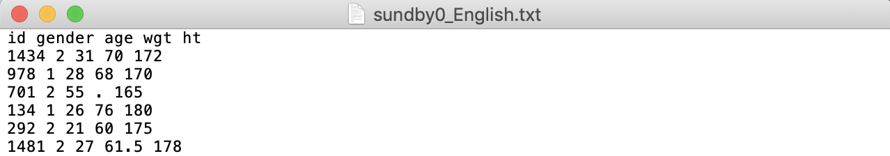
Figure 4.5: A snapshot of the SundBy text file.
To load the data into R we can use read.csv() with additional arguments. Some of the additional arguments to read.csv() are:
read.csv( file, sep, na.strings, dec)
sep
|
The separator. Default is ",". Common alternatives are semicolon ";" or whitespace " ".
|
na.string
|
The code for missing values. Default is "NA".
|
dec
|
The character used for the decimal point. Default is ".".
|
When using read.csv() we only need to specify the additional arguments, if they differ from the default values. In the text file version of the SundBy data the separator is a whitespace, missing code and the decimal point is a period. The file can therefore be loaded using:
d <- read.csv( "sundby0_English.txt", sep=" ", na.strings=".")Again we examine whether data were properly loaded, e.g. by studying the structure:
> str( d )
'data.frame':   200 obs. of  5 variables:
 $ id    : int  1434 978 701 134 292 1481 1272 1007 3 1425 ...
 $ gender: int  2 1 2 1 2 2 2 2 1 1 ...
 $ age   : int  31 28 55 26 21 27 65 79 37 36 ...
 $ wgt   : num  70 68 NA 76 60 61.5 80 60 75 83 ...
$ ht : int 172 170 165 180 175 178 168 172 170 183 ...Above, in Chapter 4.3, we used read.csv2() to load the Danish version of the CSV file. We may actually also load this file using read.csv() if we specify semicolon as the separator (sep) and comma as the decimal point (dec):
d <- read.csv( "sundby0_Danish.csv", sep=";", na.strings="NA", dec=',')
# We may omit na.strings:
d <- read.csv( "sundby0_Danish.csv", sep=";", dec=',')
# ... as NA is the default missing value code in R
Having loaded the data the first step is always to examine whether data were loaded correctly. In the two examples below we illustrate how to use the commands given in Chapter 4.4 to reveal that data were not properly loaded.
Error example 1
Suppose we specified the wrong separator, e.g. a comma, when loading the text file:
d <- read.csv('sundby0_English.txt', sep=",", na.strings=".")and examine the data
> head( d )
  id.gender.age.wgt.ht
1     1434 2 31 70 172
2      978 1 28 68 170
3       701 2 55 . 165
4      134 1 26 76 180
5      292 2 21 60 175
6   1481 2 27 61.5 178
> str( d)
'data.frame':   200 obs. of  1 variable:
 $ id.gender.age.wgt.ht: Factor w/ 200 levels "10 2 32 54 165",..: 68 197 158 51 91 74 40 3 92 63 ...
We note that the data are not organized in columns and that the data frame contains only one variable (named id.gender.age.wgt.ht) and value 1434 2 31 70 172 for the first row. Clearly the data were not loaded properly. Fortunately we can easily correct the error by specifying a whitespace as separator.
Error example 2
Suppose we forget to specify the missing data code (which in this file is different from the default NA used in R):
d <- read.csv("sundby0_English.txt", sep=" ")and examine the data
> str( d)
'data.frame':   200 obs. of  5 variables:
 $ id    : int  1434 978 701 134 292 1481 1272 1007 3 1425 ...
 $ gender: int  2 1 2 1 2 2 2 2 1 1 ...
 $ age   : int  31 28 55 26 21 27 65 79 37 36 ...
 $ wgt   : Factor w/ 57 levels ".","100","102",..: 32 29 1 39 20 22 43 20 38 46 ...
 $ ht    : Factor w/ 42 levels ".","148","150",..: 21 19 14 29 24 27 17 21 19 32 ...
We note that we have 5 variables as expected but that the weight and height variable are registered as factor variables, namely categorical variables with text values (learn more about factors in Chapter ?? EJ LAVET). This is because these two variables have missing values and we have not told that the missing value code is a period. Instead R thinks the period is a text string. We therefore will not obtain any summary statistics for these two variables using the summary() command as R will not determine the mean etc. for categorical variables:
> summary( d )
       id             gender           age             wgt
 Min.   :   3.0   Min.   :1.000   Min.   :18.00   70     : 16
 1st Qu.: 426.2   1st Qu.:1.000   1st Qu.:27.00   65     : 11
 Median : 785.5   Median :2.000   Median :35.00   75     : 11
 Mean   : 793.1   Mean   :1.555   Mean   :41.08   59     :  8
 3rd Qu.:1194.8   3rd Qu.:2.000   3rd Qu.:53.25   72     :  8
 Max.   :1508.0   Max.   :2.000   Max.   :87.00   78     :  8
                                                  (Other):138
       ht
 170    : 19
 172    : 15
 178    : 11
 160    :  9
 167    :  9
 176    :  9
 (Other):128
Instead R tabulates six of the values of these variables. Also note that the weight variable wgt has no missing values (otherwise a line with the number of NAs would be seen in the summary) as "." is considered as a (text) value and not a missing.
4.6 Loading data from web
It is also possible to load text and CSV files into R directly from the web using read.csv() or read.csv2(). As above you need to be aware of whether the files are saved in English or Danish format and the missing value code. Copy the link to the file (from https://publicifsv.sund.ku.dk/~sr/intro/datasets/ right click on the file and choose ‘Copy link’), for example sundby0_English.csv, and paste the link instead of the filename into read.csv():
d <- read.csv("http://publicifsv.sund.ku.dk/~sr/intro/datasets/sundby0_English.csv")This way of loading data is convenient as you do not have to load the data to your folder or set the working directory. Many of the data sets we use for teaching are saved on a homepage as CSV or text files. However some computers (RegionH!) might have a problem with the security certificate on our webpages in which case data cannot be loaded directly from the web.
Exercise
Also load the other two SundBy data files (sundby0_danish.csv and sundby0_English.txt) directly from the web by modifying the code above, namely by using read.csv2() or specifying additional arguments to read.csv() depending on which file you are loading.
Solution
# Loading the Danish version of the file we simply use read.csv2()
d <- read.csv2("http://publicifsv.sund.ku.dk/~sr/intro/datasets/sundby0_Danish.csv")

# Loading the text file we use additional arguments
d <- read.csv("http://publicifsv.sund.ku.dk/~sr/intro/datasets/sundby0_English.txt",
              sep = " ", na.strings = ".")
You may skip the remaining two subchapters as the contents are Nice-to-Know for your future work with R rather than Need-to-Know.
4.7 Loading Excel files
It is also possible to load an Excel file (xls or .xlsx) into R. Loading an Excel file is not integrated in the standard version of R but the package named readxl contains a function to load Excel files easily.
You first need to install the readxl package by typing
install.packages('readxl')in to the console window. Choose a mirror close to your geographical location (Denmark) in the pop-up box. The package is installed if the message in the consol window is ended with The downloaded binary packages are in … ‘some folder with a strange name’.
The functions in the downloaded package can now be made available using
library( readxl )Open one of the CSV files in Excel (use the Danish (English) file if you have the Danish (English) version of Excel). Save the file as an Excel-projektmappe / Excel-workbook (.xlsx) named sundby0.xlsx in the same folder.
You can now load the Excel data file into R using the command read_excel():
# Be aware that the file is saved in your working directory - use dir() to check!
d <- read_excel('sundby0.xlsx')
You may get a warning about a tibble package. Ignore it, it is not important. .
Investigating the loaded data, we find that the data are displayed a bit differently when using the head() command as the types of the variables are shown:
> head(d)
# A tibble: 6 x 5
     id gender   age wgt   ht
  <dbl>  <dbl> <dbl> <chr> <chr>
1  1434      2    31 70    172
2   978      1    28 68    170
3   701      2    55 NA    165
4   134      1    26 76    180
5   292      2    21 60    175
6  1481      2    27 61.5  178
The first three variables are registered as type double (dbl, numeric potentially containing decimal numbers). Note that the weight and height variables incorrectly have been registered as character variables (chr). This is due to an unusual missing value code (in Excel a field would typically be blank if missing). We therefore need to specify that these two variables should be numeric and the code for missing values. Further, we may want to define the gender variable as a character variable:
d <- read_excel('sundby0.xlsx',
                col_types = c('numeric','text','numeric','numeric','numeric'),
                na='NA' )
Note that we have to specify the types (col_types argument) for all the five variables in our data set (if you have many variables this may be a bit cumbersome). The variables are now registered as:
> head(d)
# A tibble: 6 x 5
     id gender   age   wgt    ht
  <dbl>  <chr> <dbl> <dbl> <dbl>
1  1434      2    31  70     172
2   978      1    28  68     170
3   701      2    55  NA     165
4   134      1    26  76     180
5   292      2    21  60     175
6  1481      2    27  61.5   178
You can find more details on the arguments to read_excel() here or using help (?read_excel or help(read_excel)).
You will have to run the library( readxl ) every time you need the read_excel command if you have closed down RStudio in the mean time as R forgets about the loaded packages. You do not have to install the package again.
NB: There are several other packages with functions to load Excel files. Our experience with these packages is not very good. We currently are not very experienced with the readxl package but has the impression that it seems to work well.
Having an Excel file you wish to load in to R you can also save the data file in CSV format using the menu in Excel (Files -> Save As, choose .csv). Next load the CSV file in to R as described in the previous Section 4.3.
4.8 Export of data files
A data set in R can be exported to other data file formats allowing the data to be used in another program also. The function write.csv() exports a data frame to a CSV file in your working directory. The syntax is:
write.csv( x, file, row.names = FALSE, quote = FALSE )Here x is a data frame or a matrix (e.g. our SundBy data set named d above), file is a character string specifying the file name (e.g. ‘sundby0.csv’,the file should have extension .csv). The argument row.names = FALSE prevents row names to be written in an additional column and quote = FALSE ensures that text values and variable names are not surrounded by quotes.
To export the kids data set considered in Chapter 3.3 to a CSV file the following commands
kids <- data.frame( subject = c(1,2,3,4),
                    gender = c("F","M","F","M"),
                    age = c(7, 5, 9, 2))
write.csv(kids, file = "kids.csv", row.names = FALSE, quote=FALSE)
will result in a file named kids.csv in the working directory. Copy the above lines to your session and open the file in Excel (locate it in your data folder (working directory)). If you have the Danish version of Excel, replace write.csv() with write.csv2() (do not change any of the arguments).